

Connect data and sites
Record consumption and activities by site. Structured categories help your team identify missing information and improve the data behind your footprint.
From purchasing data and energy bills, be2morrow automatically calculates your company's Scope 1, 2 and 3 emissions and writes the report for auditors, banks and customers. Set it up once and it stays up to date.
Enter data, understand emissions, plan measures. Three building blocks that work together.
Example views with demo data.
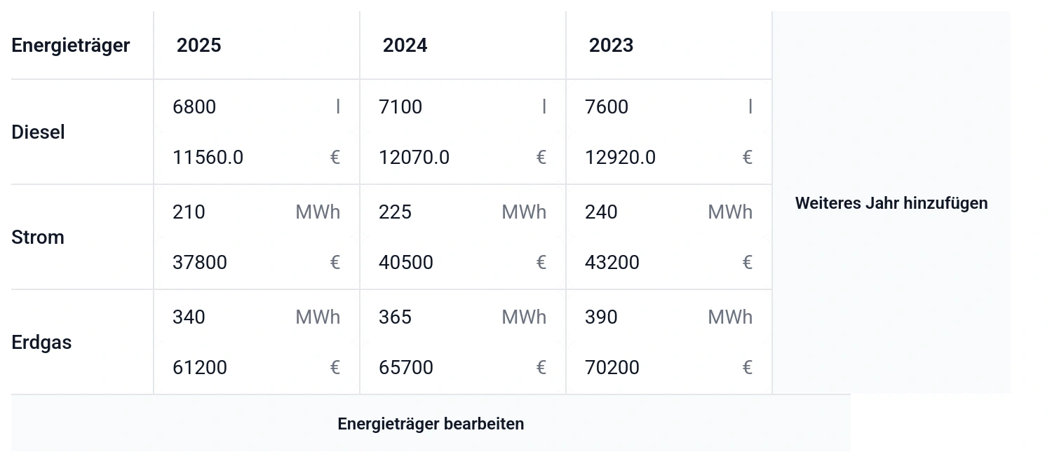
Electricity, heat and fuels: record consumption at your sites across multiple years.
Site data forms the basis of your corporate carbon footprint. This example shows data entry for a production site.
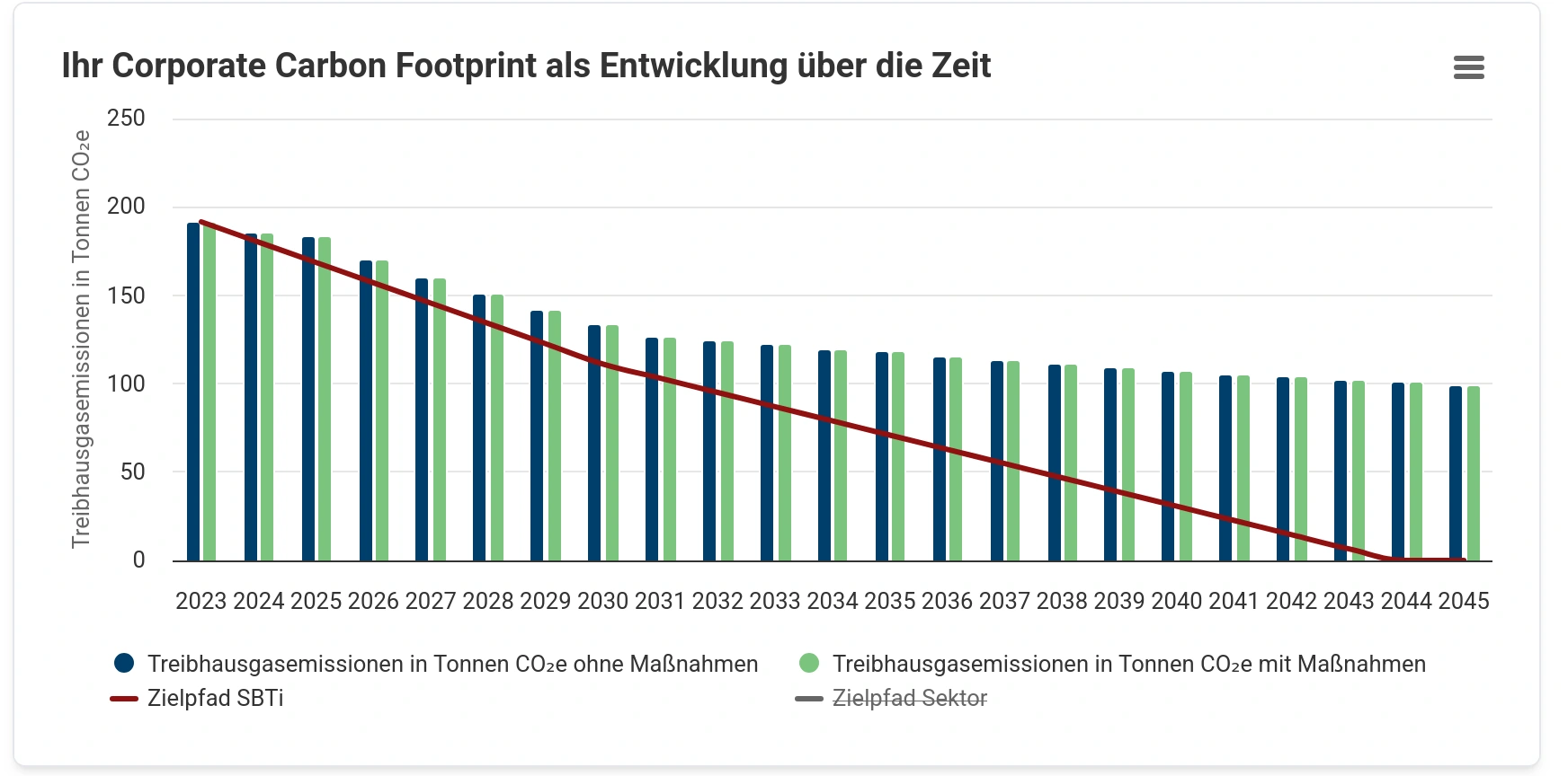
The carbon footprint brings your emissions together. The timeline shows where your company stands and how emissions are projected to develop.
Compare the forecast with your target pathway to identify where further measures are needed.
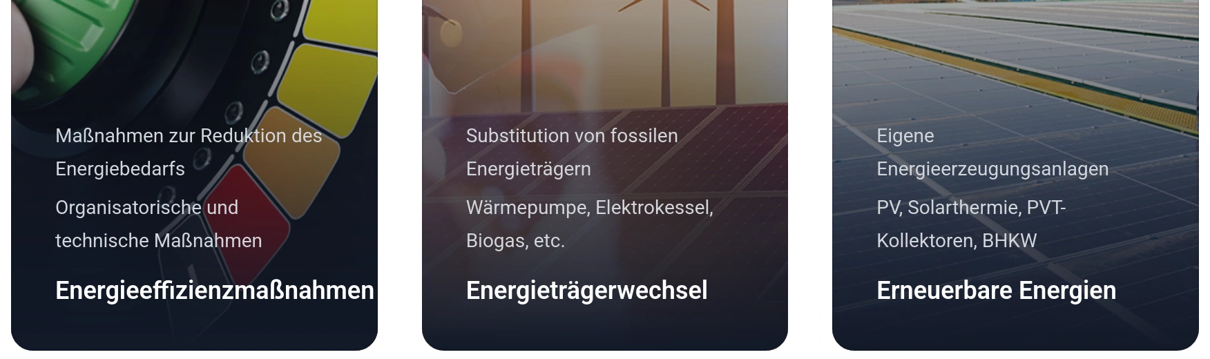
From saving energy to generating your own: put together measures that suit your business.
The platform offers different types of measures. Your chosen measures feed into your planning.
From the first data point to the next measure: organise carbon accounting so your team can keep moving forward.
Record consumption and activities by site. Structured categories help your team identify missing information and improve the data behind your footprint.
Explore emissions by scope and category. Compare their contributions to the total and use the results as a basis for your climate strategy.
Keep track of measures, responsibilities and progress. Turn your footprint into a working basis for decisions and ongoing reporting.
The platform connects an understanding of your emissions with concrete measures. Three perspectives on the same decision.
Consistent worked example: fictional industrial company, inventory year 2026. No customer data.
Which sources shape your inventory? Look at the distribution across scopes and investigate the biggest opportunities.
| Emission scope | t CO₂e | Share |
|---|---|---|
| Scope 1 | 412.8 | 14.5 % |
| Scope 2 | 398.6 | 14.0 % |
| Scope 3 | 2,036.2 | 71.5 % |
As in the platform dashboard: compare annual emissions with and without measures as paired bars. The line shows the target pathway.
Annual emissions · t CO₂e
| Year | Without measures | With measures | Your climate target |
|---|---|---|---|
| 2026 | 2,847.6 | 2,847.6 | 2,847.6 |
| 2027 | 2,873.2 | 2,634.7 | 2,591.3 |
| 2028 | 2,899.1 | 2,412.8 | 2,335.0 |
| 2029 | 2,925.2 | 2,168.5 | 2,078.7 |
| 2030 | 2,951.5 | 1,976.3 | 1,822.4 |
| 2031 | 2,978.1 | 1,814.9 | 1,566.2 |
Which climate measure pays off, and under which assumptions? Our VALERI solution connects carbon impact with net present value, discounted payback and carbon abatement costs. Comparing scenarios supports a better-informed decision.
Reduce emissions and make informed investment decisions: compare options, review assumptions and see how sensitive the result is to costs and energy prices.
Illustrative energy-efficiency measure: €128,000 initial investment in year 0, ten operating years and 64,000 kWh saved annually. The first-year energy price is €0.3075/kWh: €19,680 gross savings less €2,400 operating and maintenance costs gives €17,280 net cash flow. The expected case assumes annual energy price growth of 4% and operating cost growth of 2%. Annual net cash flows are discounted at 3%. Net present value equals the sum of discounted net cash flows less the initial investment.
Best case: annual energy price growth of 6%, investment and operating costs −10%, discount rate 3%. Worst case: annual energy price growth of 1%, costs +15%, discount rate 7%. Operating costs grow by 2% annually in every scenario. Annual price changes compound; discounting works against this growth. Discounted payback is interpolated between annual values. Excludes taxes, subsidies and residual value. All price assumptions are illustrative, not forecasts.
Cumulative discounted cash flow · € thousand
Each curve starts with the negative initial investment. Expected discounted cash flow turns positive in operating year 8; worst-case net present value remains negative after ten years.
Payments and cash flow · expected, € thousand · nominal
Bars show the investment in year 0 and annual net savings. The line adds up these payments: cumulative cash flow becomes positive in operating year 7. Both series are nominal, without discounting.
| Year | Gross savings · expected | Cash flow · nominal | Cash flow · discounted | Cumulative nominal cash flow | Best case | Expected | Worst case |
|---|---|---|---|---|---|---|---|
| 0 | — | -128,000 € | -128,000 € | -128,000 € | -115,200 € | -128,000 € | -147,200 € |
| 1 | 19,680 € | 17,280 € | 16,777 € | -110,720 € | -98,190 € | -111,223 € | -131,387 € |
| 2 | 20,467 € | 18,019 € | 16,985 € | -92,701 € | -80,604 € | -94,238 € | -116,485 € |
| 3 | 21,286 € | 18,789 € | 17,195 € | -73,912 € | -62,424 € | -77,044 € | -102,441 € |
| 4 | 22,137 € | 19,590 € | 17,406 € | -54,321 € | -43,635 € | -59,638 € | -89,207 € |
| 5 | 23,023 € | 20,425 € | 17,619 € | -33,896 € | -24,220 € | -42,019 € | -76,736 € |
| 6 | 23,944 € | 21,294 € | 17,833 € | -12,603 € | -4,161 € | -24,186 € | -64,984 € |
| 7 | 24,901 € | 22,199 € | 18,050 € | 9,596 € | 16,559 € | -6,136 € | -53,909 € |
| 8 | 25,898 € | 23,141 € | 18,267 € | 32,737 € | 37,961 € | 12,131 € | -43,474 € |
| 9 | 26,933 € | 24,121 € | 18,487 € | 56,858 € | 60,061 € | 30,618 € | -33,642 € |
| 10 | 28,011 € | 25,143 € | 18,708 € | 82,001 € | 82,881 € | 49,327 € | -24,377 € |